Virtually all spreadsheet software offers a way to create pie charts. Today we’ll focus on creating pie charts in Microsoft Excel.
How to Create a Pie Chart in Excel
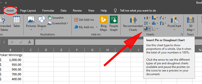
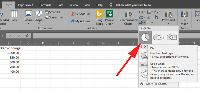
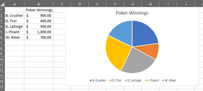
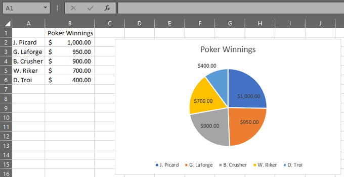
Microsoft Excel is the gold standard of office spreadsheet software. We’ll be using the desktop application, but you can opt to use the web version. After all, the Microsoft Office suite for the web is available for free! Let’s look at how to create a pie chart from your data in Excel. You have just created a pie chart! Next we’ll explore adjusting the look and feel of your pie chart.
Formatting Your Pie Chart
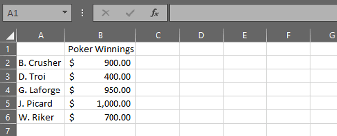
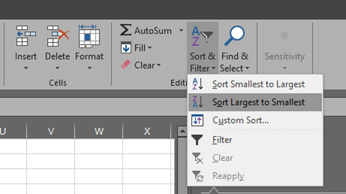
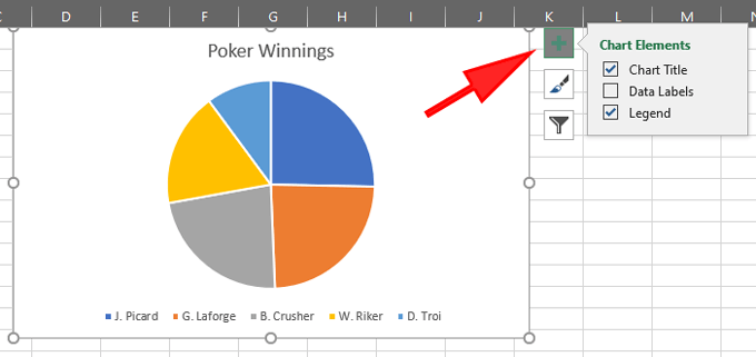
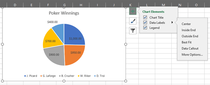
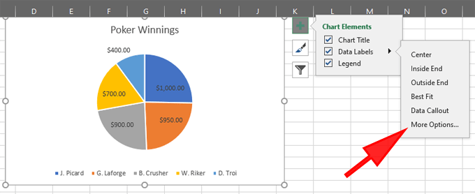
Excel offers several ways to format pie charts. You can change the Chart Title if you like. Excel automatically uses the header of the column where your chart data is stored—in this case, “Poker Winnings.” If you update the text of that column’s header, the pie chart’s title will update automatically. Alternatively, you can double-click on the chart title itself and edit it. You should also put your data in the right order. Imagine an analog clock superimposed on top of your pie chart. The biggest slice of the pie should begin at 12:00. As you go clockwise around the pie, the slices should get progressively smaller. In order to accomplish this, you need to sort your numerical data from largest to smallest. Select the Home menu item. Make sure your cursor is in one of the cells in the column with numerical data. Select the Sort & Filter button on the ribbon and choose Sort Largest to Smallest. Your pie chart will automatically update, and now you’re following best practices regarding the order of your data within the pie chart. Choose your Data Labels. Begin by clicking on the pie chart and selecting the green plus icon to the right of the chart to display Chart Elements. Now check the box next to Data Labels. Expand the options for Data Labels and then select More Options… That will open the Format Data Labels panel.
How Excel Pie Chart Labels Work
The Format Data Labels panel is where you can choose which labels will appear on your pie chart. Select the bar graph icon called Label Options. Expand the Label Options section and you’ll see a number of labels you can choose to display on your pie chart. Here’s how each label option works:
Value from Cells: In the example above, the pie chart displays one column of data. If you had another column of data, you could use this option to use those values when labeling each slice of the pie. In other words, you can choose to use the data from a different range of cells as your data labels. For example, you can add a third column to your data, “Change from last week.” If you choose value from cells and select cells C2:C6, then your pie chart would look like this:
Series Name: Checking this option will add the heading of your data column to every slice of the pie. In our example, each slice of the pie would get a label saying “Poker Winnings.”Category Name: This one is recommended. Instead of having to refer to the legend, this option will label each slice of the pie with the category values.Value: This is checked automatically. Each slice of the pie is labeled with the data value corresponding to that slide. In our example, that’s the dollar amount each poker player won.Percentage: This is often very useful. What percentage of the whole pie does the slice represent? Checking this box will ensure that the slice is labeled with the percentage the slice represents.Show Leader Lines: If the data label won’t fit entirely inside the slice, this option will add a line connecting the data label to the slice.Legend Key: If you don’t have Category Name enabled, be sure to check this box so the legend appears at the bottom of your pie chart.
Changing Pie Chart Colors
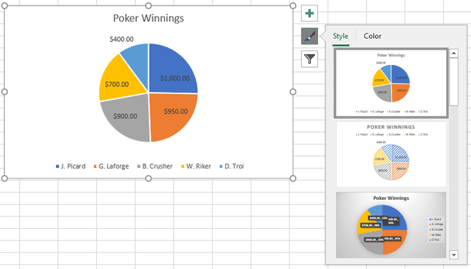
To change your pie chart color scheme, begin by selecting the pie chart. Then select the paintbrush icon, Chart Styles. You’ll see two tabs, Style and Colors. Explore the options in both tabs and choose a color scheme you like.If you want to highlight a specific slice of the pie, apply a color to that slice while choosing a shade of gray for all the other slices. You can select a single slice of the pie by selecting the pie chart and then clicking on the slice you want to format. You can also move the slice you want to highlight slightly away from the center to call attention to it like this:
Changing Pie Chart Type
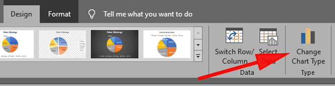
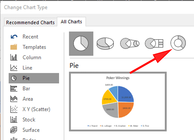
To change the chart type, select the Design tab on the ribbon and select Change Chart Type. For example, select the Donut Chart. Now our example pie chart looks like this:
Other Kinds of Charts in Excel
Now that you know the basics of creating a pie chart in Excel, check out our article, “Charting Your Excel Data” to learn more tips and tricks on how to present your data visualizations in clear, compelling ways.